In order to optimise the gas production and for better understanding the liquid loading problem, a method has been developed that enables the simulation of the fluid temperature during production. The approach incorporates complex wellbore geometry and wellbore completion as well as modelling the transient behaviour of the layered geology surrounding the borehole. The model is separated into two parts, a steady state borehole model and a transient earth model, which are connected via the borehole wall temperature. The steady state borehole model is responsible for the calculation of the fluid temperatures along the borehole trajectory, whereas the earth model considers the behaviour of the surrounding formations by use of transient heat conduction functions based on infinite line source and cylindrical heat source models.
Conventional solutions for both models incorporating a linear geothermal gradient have been discussed and published widely, but the major constraint of all those methods is that the borehole conditions need to be homogeneous. The new approach separates the borehole into numerous vertical sections. The adjoining sections are concatenated by using the fluid temperatures at the end of the section as boundary conditions for the governing differential equations.
The complete model finally includes conduction and radiation models to handle heat transfer through mechanically as well as vacuum or gas insulated tubing and through the annulus. Convective heat transfer models based on the Nusselt, Prandtl and Reynolds number are applied to quantify the heat transfer coefficients for both free and forced convection. Combining such a wellbore heat transfer model with sophisticated models for liquid loading, yields on the one hand a better understanding of what is happening in the borehole, and on the other hand allows a more accurate prediction of critical events.
1 Introduction
Since heat and thus thermal energy is ubiquitous, the understandings of heat behaviour as well as the transfer mechanisms in a borehole are important and responding to a growing interest. Especially in the field of crude oil and natural gas production, numerous attempts have been made to create and/or use appropriate models to refine knowledge. Kunz and Tixier (1) created a wellbore temperature model for the interpretation of temperature curves recorded in gas producing wells. Elshahawi et al. (2) used heat transient transfer models for supporting interpretation of both, build-up and draw-down testing of gas wells. Pigott et al. (3) applied heat transfer models to understand and quantify the effect of wellbore heating as counteraction to liquid loading.
Ipek et al. (4) showed that temperature logs can be used to identify entry and exit points of underground blowouts. They presented a model relating underground rate and the flowing fluid temperature that is valid for short flow-time. Application of that method was illustrated for hypothetical as well as for two real world examples. Michel and Civan (5, 6) developed an improved non-isothermal mathematical model considering the non-equilibrium effects involved during rapid multiphase flow in wells. They showed applications for two and three phase systems and claimed that their model can be coupled with reservoir simulation for accurate representation of the well-fluid hydraulics under non-equilibrium and non-isothermal flow conditions. Izgec et al. (7, 8) present two methods for estimating flow rates, predominantly from temperature data to complement rate measurements. One approach consists of modelling the entire wellbore and requires both wellhead pressure and wellhead temperature, whereas the other uses transient temperature formulation at a single point in the wellbore to compute the total production rate.
Barret et al. (9, 10, 11) presented an algorithm for determining gas flow rate and thermal conductivity values of the formation from pressure and temperature profiles in vertical wells. They validated the proposed method by comparing measured and calculated temperature and pressure profiles as well as their flow rate prediction with flowmeter data obtained by production logging tools. The thermal conductivity values also showed good agreement with the data obtained from lithology logs.
2 Theory
2.1 Removal of liquids in gas wells
During gas production, liquids like water or condensates are almost always present. These liquids may either occur in the reservoir and be produced along with the gas, or they may start to appear due to condensation. These liquids have to be transported by the gas up to the surface. However, since the gas flow rates will decline over time and thus the flow velocity of the gas will be reduced, the velocity will eventually drop below a certain minimum value. Once this happens, the liquids will not be carried to the surface but rather start to accumulate at the bottom of the borehole. This liquid accumulation creates a backpressure which will at the least hinder gas production and in the worst case, completely stop the gas flow from the formation altogether (12).
Turner et al. (12) were the first to investigate liquid loading and how to prevent it by calculating a minimum flow rate. They analysed two different models: the continuous film model, which describes the movement of liquid along the pipe wall due to shear forces, and the entrained droplet model, which characterizes the liquid drops moving upward as a result of drag forces. The conclusion was that the flow velocity has to exceed a certain threshold at all times to ensure a steady removal of the largest occurring drops. The balance of forces between the forces of gravity
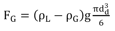 (1)
(1)
and the drag force experienced by the droplet
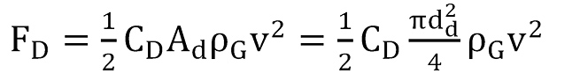 (2)
(2)
results in the so-called threshold velocity.
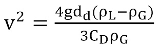 (3)
(3)
That equation is further used to determine the so-called Turner equation. To substitute the unknown diameter dd (Eq.5) of the entrained droplets and to account for the influence of velocity and surface tension, the Weber number (Eq.4) is introduced and arranged to give dd.
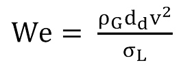 (4 )
(4 )
 (5)
(5)
After rearrangement, the formula for the critical velocity to lift droplets in vertical wells is obtained as
 (6)
(6)
In their study, Turner et al. (12) substitute drag coefficient, surface tension and liquid densities with average values. For the gas density – a function of pressure, temperature and gas gravity – average values for temperature and gas gravity were used. For the Weber number, Turner et al. (12) turned to the studies of Hinze (13) who showed that droplets shatter once they exceed a critical value of the Weber number. Hinze determined the critical Weber number Wec to be in the range of 20 to 30, and Turner et al. decided to use the larger value of Wec = 30. Thus, they arrived at two simplified final equations, for water (Eq.7) and for condensate (Eq.8), both of which are a function of pressure only.
 (7)
(7)
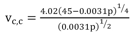 (8)
(8)
These two equations also include an upward adjustment of about 20 % which comes from the fact that Turner et al. (12) compared their results with actual field data and found that this correction was required to achieve a sufficiently good match. Coleman et al. (14) however state that they consider this adjustment to be unnecessary and that accurate prediction can be achieved without it.
Another model was conceived by Li et al. (15) who argued that the assumptions made by Turner et al. (12) concerning shape and drag coefficient of the entrained droplets are not definitive. They postulate that the droplets experience significant deformation during their upward transport through the wellbore and estimate a drag coefficient of 1.0, instead of 0.44 as used by Turner et al. (12). As a result, Li et al. (15) obtain much lower critical velocities before liquid loading occurs.
Luan et al. (16) compared these models and found that Turner’s model, including the 20 % adjustment, is best suitable for flowing wellhead pressures of 5.5 MPa or greater. Coleman’s model, which is Turner’s model without 20 % adjustment, should be used for wellhead pressures of 3.4 MPa or less. However, nearly all investigated gas wells exhibited liquid loading well before Li’s critical flow rates were reached.
In this study, the focus lies on determining theses variables – such as the densities, surface tension, etc. – through calculations rather than estimations and thus, to ultimately achieve a reliable model.
Moreover, to make sure that the simulation of the critical velocity is not limited to vertical wells but can also be applied to increasingly more common deviated wells, a pipe angle α as shown in Figure 1 is considered which indicates the deviation from the horizontal plane.
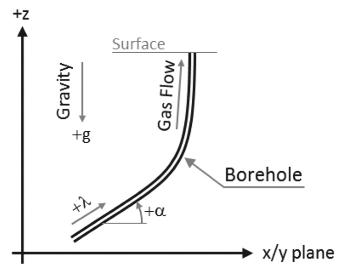
Fig. 1. Coordinate system used // Bild 1. Verwendung eines Koordinatensytems.
This angle is included in the final form of the equation (17).
 (9)
(9)
2.2 Heat Transfer in Boreholes
The derivation of the general equations for temperature and pressure prediction in a borehole is based on the conservation laws of mass, momentum and energy, e. g., Michel and Civan (5, 6).
The mass balance enables to define that the mass flow rate within the borehole does not change.
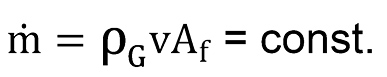 (10)
(10)
Using local coordinates as sketched in Figure 1, the equation for pressure is obtained by momentum balance as
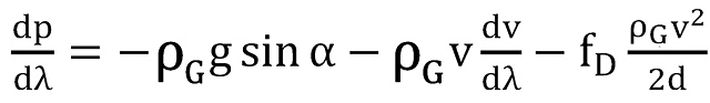 (11)
(11)
and the temperature equation can be written by combining mass and energy balance
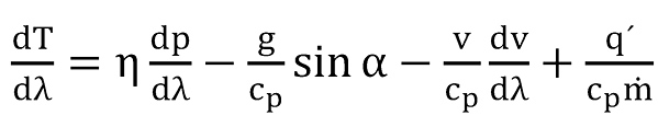 (12)
(12)
It is obvious that above equations depend on each other since gas density, heat capacity, viscosity and Joule- Thompson coefficient among others depend themselves on pressure and temperature.
To obtain an analytical solution as far as possible, Eq.(11) and Eq.(12) have been solved assuming that above mentioned parameters are constant. The solution for the pressure can thus be written as
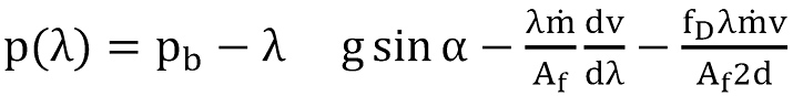 (13)
(13)
The boundary condition pb for the first section is equivalent to the pressure at reservoir depth in the casing, and for the succeeding section it is the calculated pressure p(L) at the top of the preceding section.
To get the solution for the temperature equation (12) the specific heat flow has to be replaced by
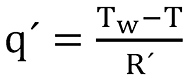 (14)
(14)
whereby the borehole wall temperature has to be replaced by the earth temperature taking care of the geothermal gradient λγe and therefore
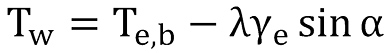 (15)
(15)
The final solution for the temperature equation can thus be written as
 (16)
(16)
The first item at the right side of above equation is the Joule-Thompson term, given by
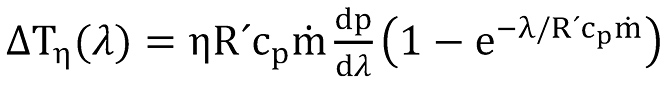 (17)
(17)
the second item is the gravity term, given by
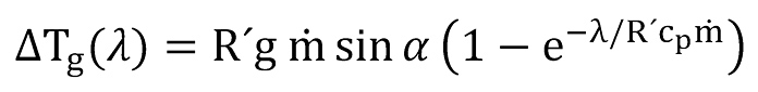 (18)
(18)
the third item is the acceleration term, given by
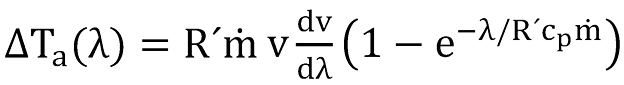 (19)
(19)
and the last term is responsible for the heat transfer with the formation,
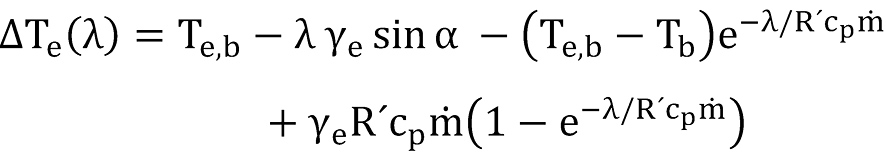 (20)
(20)
The overall thermal resistance is calculated as the sum of all thermal resistances between the inside of the pipe and the borehole wall (Figure 2).
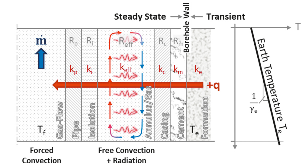
Fig. 2. Cross-section of borehole. // Bild 2. Bohrlochquerschnitt.
It includes all resistances caused by conduction, convection as well as radiation. The heat transfer coefficient due to forced convection is based on the Nusselt number; we used the correlation published by Gnielinski (18). The resistance due to free convection of the annular gas is calculated by the Dropkin & Somerscales correlation (19) using Grashof number and Prandtl number.
Since the specific thermal resistance is given by R´=R L, the overall thermal resistance can be expressed as the sum of the specific resistances of the pipe, the annulus, the borehole completion and another term responsible for the transient modelling, denoted as H´(t).
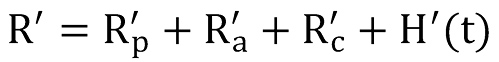 (21)
(21)
The last term in above equation can be considered as a time dependent specific resistance which is responsible for the transient behaviour of the formation. H´(t) can be expressed by the so-called transient heat conduction function g(t) which is sometimes denoted as g-function.
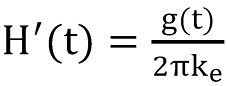 (22)
(22)
The g-function can be considered as a source or sink in an infinite body and has the advantage that transient models can be established without stepping into numerical simulations. The transient earth model is thereby usually linked via the borehole wall temperature to the steady state borehole model. Solutions for the transient heat conduction function applicable to boreholes are available as infinite line source and as cylindrical heat source models (20).
To obtain further the final solutions for pressure and temperature in the borehole, the borehole has been separated into sections of (possibly unequal) lengths and the above analytical solutions were used iteratively to calculate pressure and temperature until convergence has been obtained in each section. In each of those sections, the thermal resistances as well as all other relevant parameters like density are repeatedly calculated at the bottom and at the top of the section.
Since the boundary conditions (BC) have been defined as pressure and temperature at the bottom of the sections (Figure 3), the calculation is done section by section.
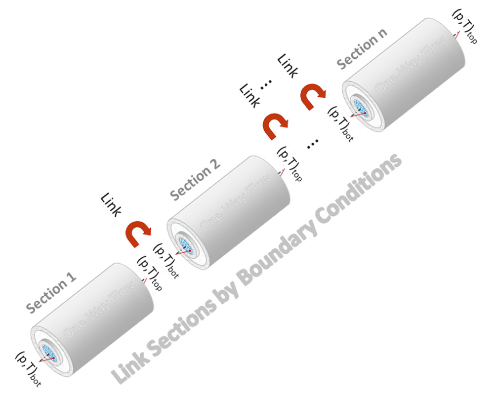
Fig. 3. Sectioning of borehole. // Bild 3. Bohrlochabschnitte.
Starting with the bottom section, the BC are defined by bottom hole pressure and temperature. After finishing the iterative calculations, all values are available at section top and passed as new boundary conditions to the next section. Using smart methods for creating the sections, inhomogeneous borehole conditions like different pipe materials, borehole diameters and completions as well as the inhomogeneous surrounding geology can be handled in an elegant way.
2.3 Correlations and models
One of the challenges of this work was the estimation of the thermodynamic parameters and the application of an equation of state (EoS) for real gases.
The equation of state used for natural gases is usually based on the compressibility factor (z-factor) model of Standing & Katz (21), whereby the z-factor denotes the ratio of the actual to the ideal volume of particular moles of a real gas at a given pressure and temperature. The equation of state can thus be written as
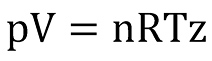 (23)
(23)
whereby the compressibility factor is usually expressed as a function of the pseudo reduced pressure and temperature z = z(ppr,Tpr). The pseudo reduced values are given by ppr = p/ppc and Tpr = T/Tpc.
Among the equation of state, other parameters are to be estimated or need to be known:
- molar mass of gas;
- pseudo critical pressure and temperature;
- gas density;
- gas heat capacity;
- gas viscosity;
- Joule Thompson coefficient;
- fluid surface tension (water and/or condensate); and
- fluid density (water and/or condensate).
If the composition of a natural gas is not exactly available, the molar mass of the gas can be correlated by using the gas specific gravity as
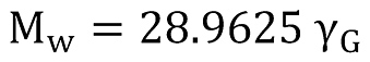 (24)
(24)
Since the number of moles of a substance can be expressed as n = m / Mw, the density of the natural gas can be calculated as
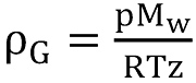 (25)
(25)
The pseudocritical values can be estimated by the Sutton correlation (22, 23), which is valid for gases free of contaminants, as
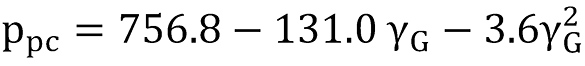 (26)
(26)
 (27)
(27)
Sutton also provides a summary of correlation models for gases containing H2S, CO2 and N2.
For the z-factor estimation, several correlations (20) are sufficiently published, e. g., Dranchuk et al. (24) or Dranchuk & Abou-Kassem (25). Abou-Kassem et al. (26) published the FORTRAN code for both of their methods.
We used one of these algorithms – the ZSTAR routine – with the corrections proposed by Borges (27) for high gas density and our own corrections for improvement of the model for low pseudo reduced pressure values (Figure 4).

Fig. 4. Used z-factor model. // Bild 4. Das verwendete z-Faktor Modell.
Expressing the heat capacity based on an equation of state is the general method in industry (28). The estimation of the ideal isobaric heat capacity of real gases has been extensively studied.
Numerous authors have presented correlations for pure compounds as well as for natural gas, but at high pressures the real heat capacity deviates from the ideal heat capacity (28). Abou-Kassem & Dranchuk (29) and Dranchuk & Abou-Kassem (30) presented a method using the EoS of Dranchuk et al. (24) to calculate heat capacity.
Lateef & Omeke (31) proposed a method using specific gas gravity and pseudo reduced pressure. In Figure 5, their heat capacity model is shown for a gas with a specific gravity of γG = 0.7.
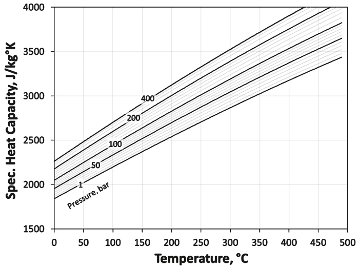
Fig. 5. Lateef & Omeke’s heat capacity model. // Bild 5. Lateef & Omeke’s Wärmekapazitätsmodell.
The viscosity of natural gas usually is in the range from 10 to 40 µPa.s at standard and reservoir conditions. The estimation of the gas viscosity is usually a two-step procedure: 1. calculating mixture low-pressure viscosity at standard pressure from Chapman-Enskog theory and 2. correcting this value for the effect of pressure and temperature with a corresponding-states or dense-gas correlation (32).
Numerous matured and well accepted models are available (33), among others Lee et al. (34), Lee & Eakin (35) or the model of Gurbanov & Dadash-Zade (36) which is shown in Figure 6 for a gas with a specific gravity of γG = 0.7.
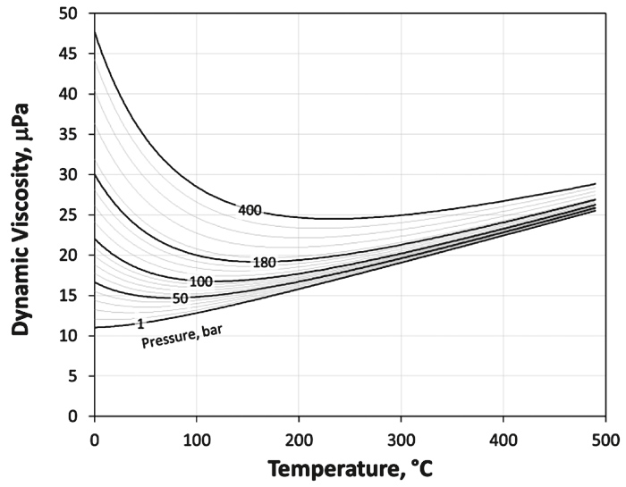
Fig. 6. Gurbanov & Dadash-Zade’s viscosity model. // Bild 6. Gurbanov & Dadash-Zade’s Viskositätsmodell.
The general expression for the Joule-Thompson coefficient can be derived from the Maxwell identities (∂H/∂p)T = V + T(∂S/∂p)T and (∂S/∂p)T =( ∂V/∂T)p, so
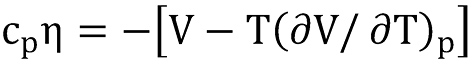 (28)
(28)
or after re-arrangement
 (29)
(29)
Since heat capacity, density and z-factor are already defined, the only challenge is the estimation of the derivative of the z-factor with respect to the temperature.
For the z-factor model shown in Figure 4, the derivatives necessary for the Joule-Thompson coefficient are calculated by numerical differentiation.
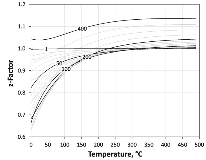
Fig. 7. z-factor vs. temperature. // Bild 7. z-Faktor vs. Temperatur.
Figure 7 shows as an example the -z-factor model for a gas with a specific gravity of γG = 0.7 and the corresponding Joule-Thompson coefficients are shown in Figure 8.
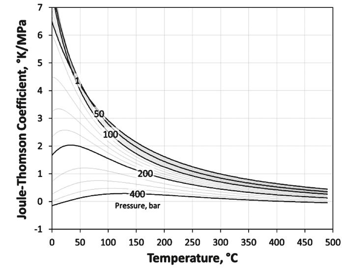
Fig. 8. Gurbanov & Dadash-Zade’s viscosity model. // Bild 8. Gurbanov & Dadash-Zade’s Viskositätsmodell.
For the surface tension Turner et al. (12) proposed using a constant value. For water they recommended a value of σH2O = 0.06 N/m. Since the surface tension is actually depending on the temperature, we used the model proposed by Kestin et al. (38) given by
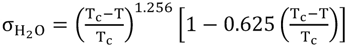 (30)
(30)
whereby Tc = 647.14 K is the critical temperature of water. The model is shown in Figure 9, and covers the entire liquid range from the triple point to the critical point.
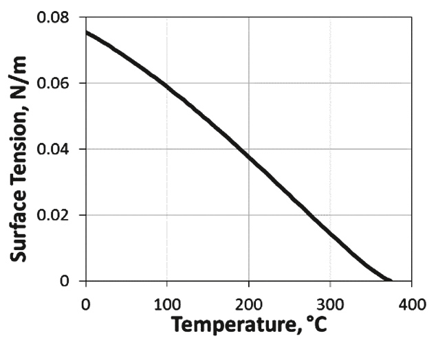
Fig. 9. Surface tension of water. // Bild 9. Oberflächenspannung von Wasser.
The model for water density we used is from the Dortmund Data Bank Software & Separation,
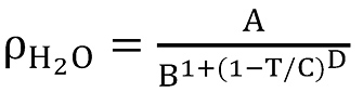 (31)
(31)
with A = 0.14395, B = 0.0112, C = 649.727, D = 0.05107 being constants.
3 Application of method
The proposed method has been applied to a borehole of 3,000 m depth drilled into a gas reservoir. The initial reservoir pressure is about 300 bar, the specific gravity of the gas is γG = 0.7.
The data of the borehole are summarized in Table 1.
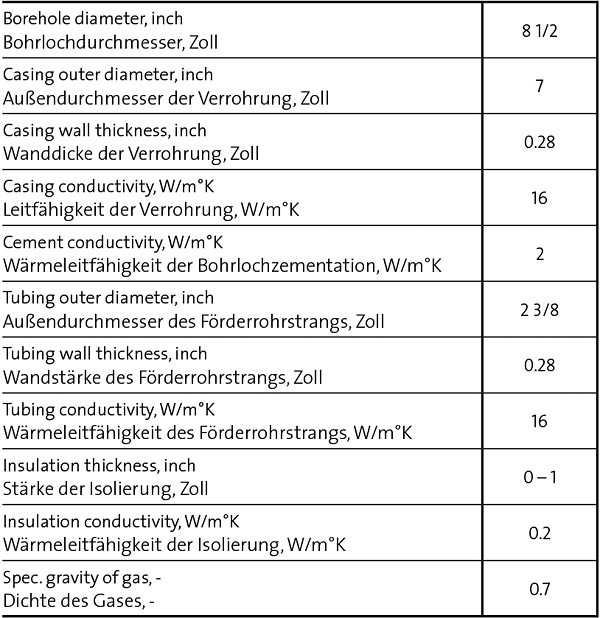
Table 1. Borehole data. // Tabelle 1. Bohrlochdaten.
Tubing and casing are made of steel, surface temperature of 15 °C is increasing by 3 °C/100m. The emissivity of tubing and casing is ε = 0.25. The simulation was done by increasing the insulation thickness from zero to 1 inch at a constant gas production rate of 100,000 Sm3/d.
The results are shown in Figure 10. The leftmost chart shows the formation temperature increasing with depth as dashed line. It can be seen that the gas temperature reduces dramatically during up-flow if the tubing is uninsulated. In this case, the temperature drops from 105 °C at 3,000m depth to about 25 °C at the surface which is a significant and irrecoverable loss of energy into the surrounding formation. This can be remedied by the use of insulation. While through the use of (unobtainable) perfect insulation, the surface temperature still reads about 89 °C, using 1 inch insulation can achieve a wellhead temperature of about 55 °C. This 30 °C increase compared to the worst case of no insulation at all constitutes a significant difference influencing relevant parameters like flow velocity.
As can be seen in the second chart of Figure 10, the occurring gas velocities exhibit noticeable variations.
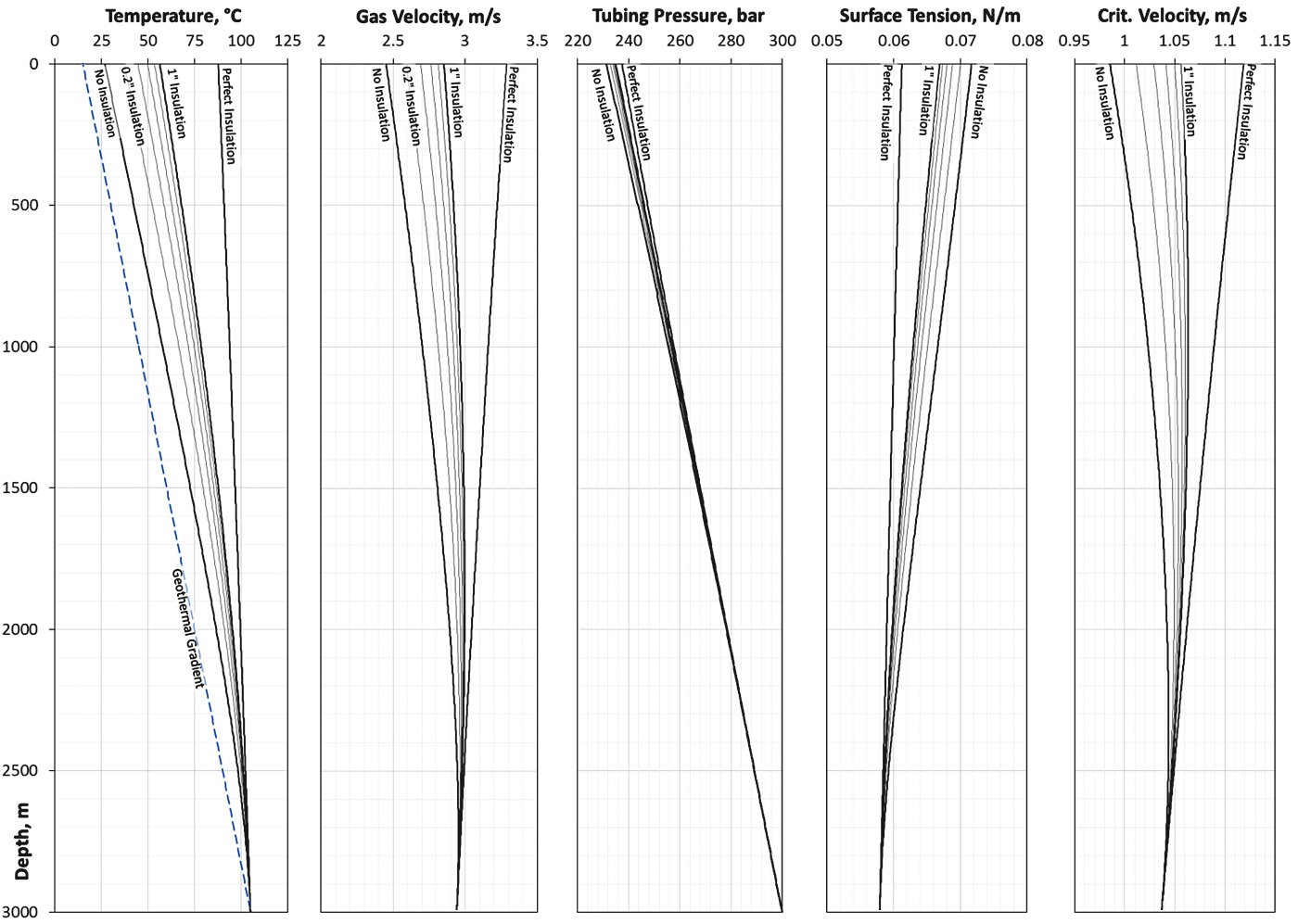
Fig. 10. Results of the simulation. // Bild 10. Ergebnisse der Simulation.
While the differences between no insulation and perfect insulation (roughly 0.9 m/s) and between no insulation and 1 inch insulation (about 0.3 m/s) may seem small, this additional velocity can be of great value especially towards the end of the lifetime of a gas well.
Another parameter influenced by insulation and additional heat energy is pressure (3rd chart in Figure 10). A variation over the range of 6 bar can be seen. Again, a higher pressure is more valuable when operating a gas well and can be obtained by sufficient insulation.
The surface tension is determined according to Eq.30 and solely depends on temperature. Thus, this parameter is sensitive to any changes caused by insulation variations.
Finally, the critical velocity (as calculated by Eq.9) varies as well. It shows that an increase in insulation efficiency also increases the critical velocity needed to lift occurring droplets by a minor amount. This critical velocity increase, however, is smaller than the velocity increase of the gas shown in 2nd chart in Figure 10.
4 Conclusion
The detailed investigation on energy conservation of the produced gas indicates an enormous potential for enhanced gas recovery. The temperature conservation eventually is the physical cause for a larger gas volume to be produced which causes higher gas velocities and therefore improved carrying capacity for liquid transportation. Finally, energy conservation will also postpone the economic limit of gas production and therefore higher recovery factors of the reservoirs are to be expected.
Tubular insulation materials are well known in oil and geothermal water production but still not popular in gas production. Further research on highly effective insulation materials is mandatory in order to optimize the efficiency of the deliquification process in gas wells.
Based upon the promising calibration results of the new simulator on field examples, the future implementation of modern materials with low heat transfer capacities will open a new dimension for enhanced gas recovery.
Nomenclature
Constants used
g … Gravitational constant g = 9.80665 m/s2
R … Ideal gas constant R = 8.3144621 J/mol°K
Symbols Used
Af … Flow area, m2
Ad … Droplet cross-section, m2
cD … Drag coefficient
cp … Specific heat capacity, J/kg°K
d … Pipe diameter, m
dd … Droplet diameter, m
fD … Darcy friction factor
FD … Drag force, N
FG … Force due to gravity, N
k … Thermal resistivity, W/ m°K
ke … Thermal resistivity of earth, W/ m°K
L … Length, m
n … Number of moles
m … Mass, kg
ṁ … Mass flow rate, kg/s
Mw … Molar mass, kg/mol
p … Pressure, Pa
pb … Pressure at bottom of section, Pa
ppc … Pseudo critical pressure, Pa
ppr … Pseudo reduced pressure
pt … Pressure at top of section, Paq´ … Specific heat flow, W/m
R … Thermal resistance, °K/W
R´ … Specific thermal resistance, m°K/W
T … Temperature, °K
Tb … Temperature at bottom of section, °K
Tc … Critical temperature, °K
Te … Earth temperature, °K
Te,b … Earth temperature at bottom of section, °K
Tf … Fluid temperature, °K
Tpc … Pseudo critical temperature, °K
Tpr … Pseudo reduced temperature
Tt … Temperature at top of section, °KTw … Borehole wall temperature, °Kv … Velocity, m/s
vc … Critical velocity, m/s
vc,c … Critical velocity of condensate droplets, m/s
vc,w … Critical velocity of water droplets
m/sV … Volume, m3
We … Weber number
Wec … Critical Weber number
z … Compressibility factor
Greek Symbols
α … Pipe angle from horizontal, deg
γG … Specific gravity of gas
γe … Geothermal gradient, °K/m
ε … Emissivity coefficient
η … Joule-Thompson coefficient, °K/Pa
λ … Length, m
μ … Dynamic viscosity, Pa.s
ρ … Density, kg/m3
ρG … Gas density, kg/m3
ρH2O … Water density, kg/m3
ρL … Liquid density, kg/m3
σH2O … Surface tension of water, N/m
σL … Surface tension of liquid, N/m
References/Quellenverzeichnis
References/Quellenverzeichnis
(1) Kunz, K. S.; Tixier, M. P.: Temperature Surveys in Gas Producing Wells. Society of Petroleum Engineers, 1955.
(2) Elshahawi, H.; Osman, M. S.; Sengul, M.: Use of Temperature Data in Gas Well Tests. Society of Petroleum Engineers, 1999. doi:10.2118/56613-MS.
(3) Pigott, M. J.; Parker, M. H.; Mazzanti, D. V.; Dalrymple, L. V.; Cox, D. C.; Coyle, R. A.: Wellbore Heating to Prevent Liquid Loading. Society of Petroleum Engineers, 2002. doi:10.2118/77649-MS.
(4) Ipek, G.; Smith, J. R.; Bassiouni, Z.: Estimation of Underground Blowout Magnitude Using Temperature Logs. Society of Petroleum Engineers, 2002. doi:10.2118/77476-MS.
(5) Michel, G.; Civan, F.: Modelling Nonisothermal Rapid Multiphase Flow in Wells under Nonequilibrium Conditions. Society of Petroleum Engineers, 2006. doi:10.2118/102231-MS.
(6) Michel, G.; Civan, F.: Modelling Nonisothermal Rapid Multiphase Flow in Wells under Nonequilibrium Conditions. Society of Petroleum Engineers, 2008. doi:10.2118/102231-PA.
(7) Izgec, B.; Hasan, A. R.; Lin, D.; Kabir, C. S.: Flow Rate Estimation from Wellhead Pressure and Temperature Data. Society of Petroleum Engineers, 2008. doi:10.2118/115790-MS.
(8) Izgec, B.; Hasan, A. R.; Lin, D.; Kabir, C. S.: Flow-Rate Estimation from Wellhead-Pressure and -Temperature Data. Society of Petroleum Engineers, 2010. doi:10.2118/115790-PA.
(9) Barrett, E.; Abbasy, I.; Wu, C. R.; You, Z.; Bedrikovetsky, P. G.: Determining Gas Flow Rate and Formation Thermal Conductivity from Pressure and Temperature Profiles in Vertical Well. Society of Petroleum Engineers, 2012a. doi:10.2118/152034-MS.
(10) Barrett, E.; Abbasy, I.; Wu, C. R.; You, Z.; Bedrikovetsky, P. G.: Direct averaging estimates of separate zone production in gas wells based on pressure and temperature profiles. Society of Petroleum Engineers, 2012b. doi:10.2118/158742-MS.
(11) Barrett, E.; Abbasy, I.; Wu, C. R.; You, Z.; Bedrikovetsky, P. G.: Determining Rate Profile in Gas Wells from Pressure and Temperature Depth Distributions. International Petroleum Technology Conference, 2013. doi:10.2523/17041-MS.
(12) Turner, R. G.; Hubbard, M. G.; Dukler, A. E.: Analysis and Prediction of Minimum Flow Rate for the Continuous Removal of Liquids from Gas Wells. Society of Petroleum Engineers, 1969. doi:10.2118/2198-PA.
(13) Hinze, J. O.: Critical Speeds and Sizes of Liquid Globules. Applied Scientific Research, Vol. 1, Issue 1, 1949, pp. 273-288.
(14) Coleman, S. B.; Clay, H. B.; McCurdy, D. G.; Norris, H. L.: A New Look at Predicting Gas-Well Load-Up. Society of Petroleum Engineers, 1991. doi:10.2118/20280-PA.
(15) Li, M.; Li, S. L.; Sun, L. T.: New View on Continuous-Removal Liquids from Gas Wells. Society of Petroleum Engineers, 2002. doi:10.2118/75455-PA.
(16) Luan, G.; He, S.: A New Model for the Accurate Prediction of Liquid Loading in Low-Pressure Gas Wells. Society of Petroleum Engineers, 2012. doi:10.2118/158385-PA.
(17) Li, J.; Almudairis, F.; Zhang, H.: Prediction of Critical Gas Velocity of Liquid Unloading for Entire Well Deviation. International Petroleum Technology Conference, 2014. doi:10.2523/IPTC-17846-MS.
(18) Çengel, Y. A.; Ghajar, A. J.: Heat and mass transfer: Fundamentals & applications. New York: McGraw-Hill, 2011.
(19) Willhite, G. P.: Over-all Heat Transfer Coefficients in Steam and Hot Water Injection Wells. Society of Petroleum Engineers, 1967. doi:10.2118/1449-PA.
(20) Carslaw, H. S., Jaeger, J. C.: Conduction of Heat in Solids. Oxford Science Publications, 1946. ISDN 0198533683, 9780198533689.
(21) Kumar, N.: Compressibility Factor for Natural and Sour Reservoir Gases by Correlations and Cubic Equations of State. Master’s thesis, Texas Tech University, Lubbock, TX, USA, 2004, pp. 10 – 11.
(22) Sutton, R. P.: Fundamental PVT Calculations for Associated and Gas-Condensate Natural Gas Systems. Society of Petroleum Engineers, 2005. doi:10.2118/97099-MS.
(23) Sutton, R. P.: Fundamental PVT Calculations for Associated and Gas/Condensate Natural-Gas Systems. Society of Petroleum Engineers, 2007. doi:10.2118/97099-PA.
(24) Dranchuk, P. M.; Purvis, R. A.; Robinson, D. B.: Computer Calculation of Natural Gas Compressibility Factors Using the Standing and Katz Correlation. Petroleum Society of CIM, Paper No. 73 – 112, 1973.
(25) Dranchuk, P. M.; Abou-Kassem, J. H.: Calculation of z-factors for natural gases using equations of state. The Journal of Canadian Petroleum Technology, July-September 1975, pp. 34 – 36.
(26) Abou-Kassem, J. H.; Mattar, L.; Dranchuk, P. M.: Computer calculations of compressibility of natural gas. The Journal of Canadian Petroleum Technology, Vol. 29, 1990, pp. 105 – 108.
(27) Borges, P. R.: Correction improves z-factor values for high gas density. Oil & Gas Journal, Vol.55, 1991.
(28) Jarrahian, A.; Karami, H. R.; Heidaryan, E.: On the isobaric specific heat capacity of natural gas. by Jarrahian, Azad in: Fluid phase equilibria: an international journal (Amsterdam: Elsevier), Vol. 384, 2014, pp. 16 – 24.
(29) Abou-Kassem, J. H.; Dranchuk, P. M.: Isobaric Heat Capacities of Natural Gases at Elevated Pressures and Temperatures. SPE Paper 10980, 1982.
(30) Dranchuk, P. M.; Abou-Kassem, J. H.: Computer calculation of heat capacity of natural gases over a wide range of pressure and temperature. Can. J. Chem. Eng., 70, 1992, pp. 350 – 55. doi:10.1002/cjce.5450700220.
(31) Lateef, A. K., Omeke, J.: Specific Heat Capacity of Natural Gas; Expressed as a Function of Its Specific Gravity and Temperature. Society of Petroleum Engineers, 2011. doi:10.2118/150808-MS.
(32) Whitson, C. H.; Brule, M. R.: Gas and Oil Properties and Correlations. Phase Behaviour, Vol. 20, SPE Monograph, SPE, Richardson, TX, 2000. ISBN 1-55563-087-1.
(33) Chen, Z. A.; Ruth, D. W.: On Viscosity Correlations of Natural Gas. Petroleum Society of Canada, 1993. doi:10.2118/93-02.
(34) Lee, A. L.; Gonzalez, M. H.; Eakin, B. E.: The Viscosity of Natural Gases. SPE Paper 1340, 1965.
(35) Lee, A. L.; Gonzalez, M. H.; Eakin, B. E.: The Viscosity of Natural Gases, Society of Petroleum Engineers, 1966. doi:10.2118/1340-PA.
(36) Gurbanoy, R. S.; Dadash-Zade, M. A.: Calculations of Natural Gas Viscosity under Pressure and Temperature. Azerbaijianskoe Neftianoe Khoziaistvo., No. 2, 1986, pp 41 –44.